
Introduction
not a tutorial, just a devlog
In my last devlog, I tried to model a 3d planet with procedural generation. This time, I want to create a fantasy map, so 2D, still using our handy voronoi graphs, but using wave function collapse instead of perlin noise. I will be using the zig programming language and ofc, raylib for rendering.
Voronoi, yet again
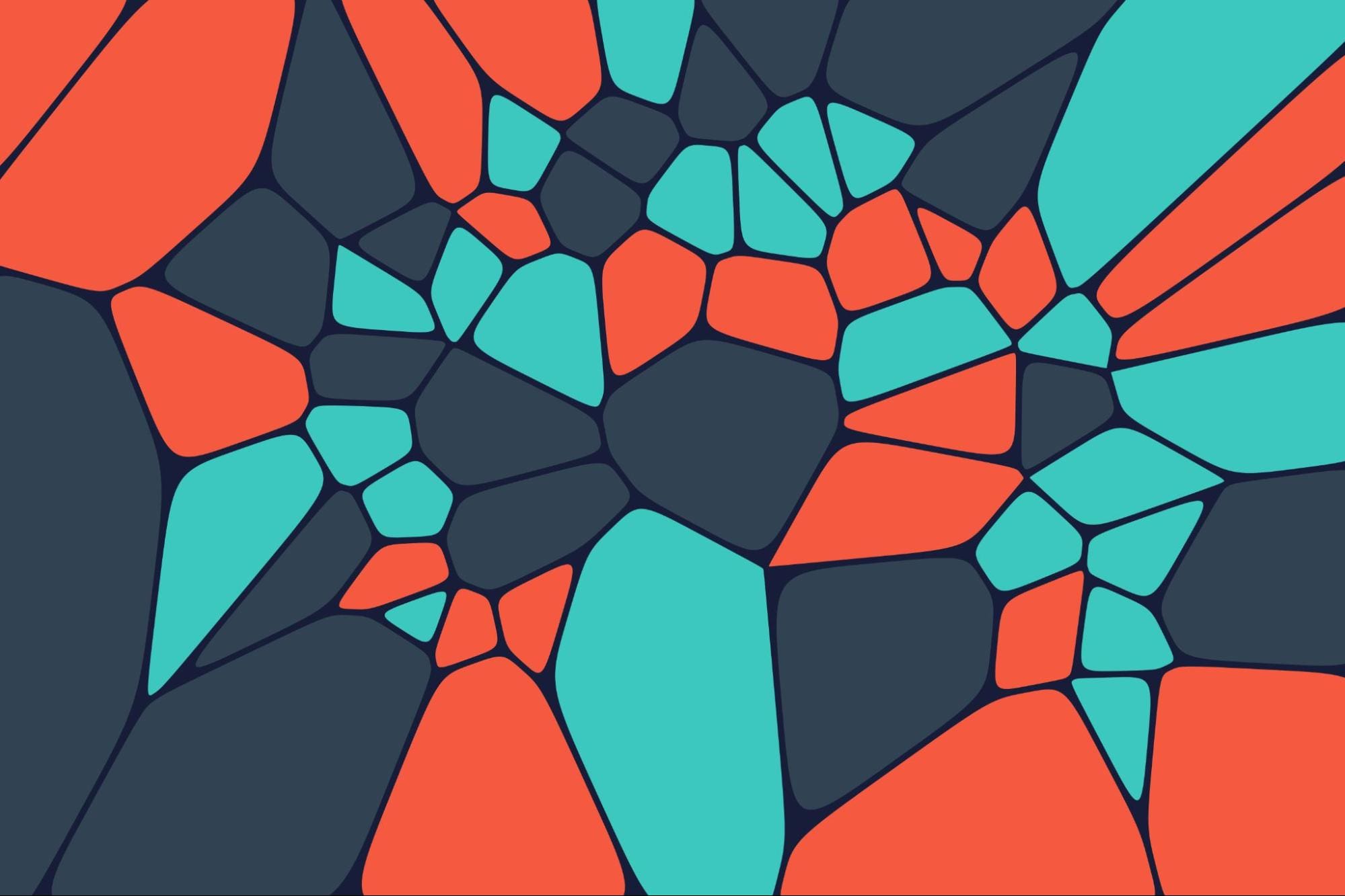
Now, in case, you have not read my previous devlog, voronoi is simply a way to divide a space into regions based on distance to a set of points. We choose a set of points, and then for each point in the space, we find the closest point from the set. This way, we can create regions that are defined by the distance to the points.
Simple beginnings
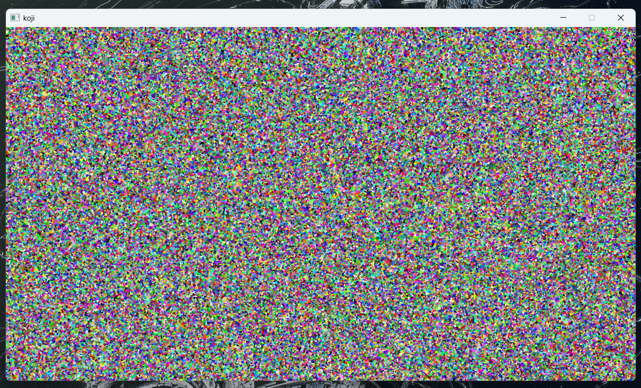
The first version of voronoi, was the most basic one, where I simply chose 150 random points, and then for each frame, I would iterate over each pixel in the screen, and find the closest point from the set.
And, I don't think I need to justify why this is not a good idea, but I will anyways. First of all, I just want a static map, so it really does not make sense to loop over each pixel every frame. Second of all, this is really slow, and it took 12.74 seconds to generate a 1280x720 map with 15 points, and it lagged so much, I could not even take a screenshot. And in the real simulation, I would be needing a WHOLE lot more points, so this is not going to work. Time for me to find out a better way.
Using a texture
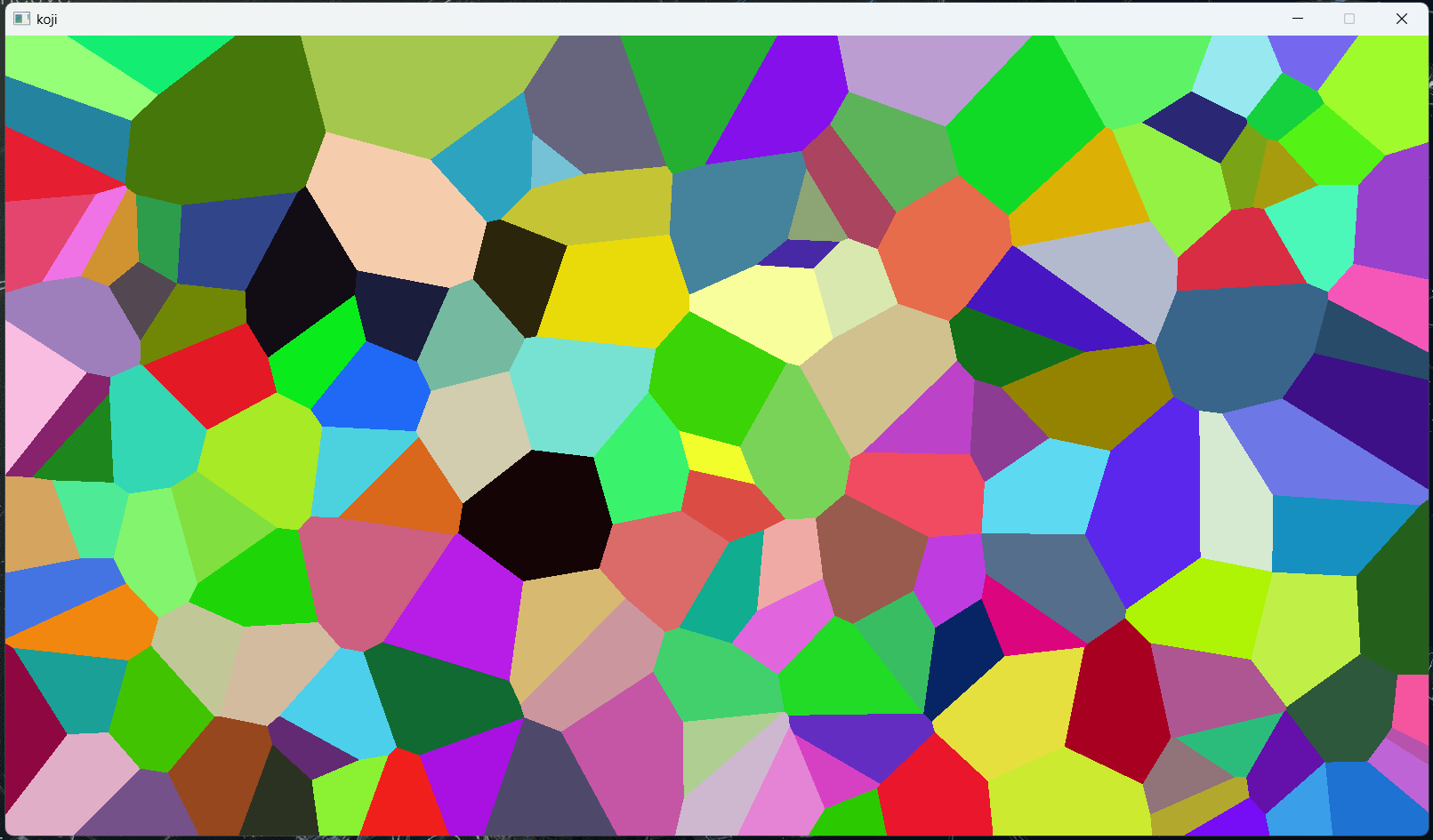
Raylib, lets us define textures, which are just array of pixels. You can use beginTextureMode and endTextureMode to draw to a texture, and then use that texture as a background. This is optimal for our use case, because we just simply want to draw the map once. This is still great, and it allowed me to atleast take a screenshot, but it still does take 12 seconds to generate a 150 point map, which is, in simple words, trash. So, I need to find a way to make this faster.
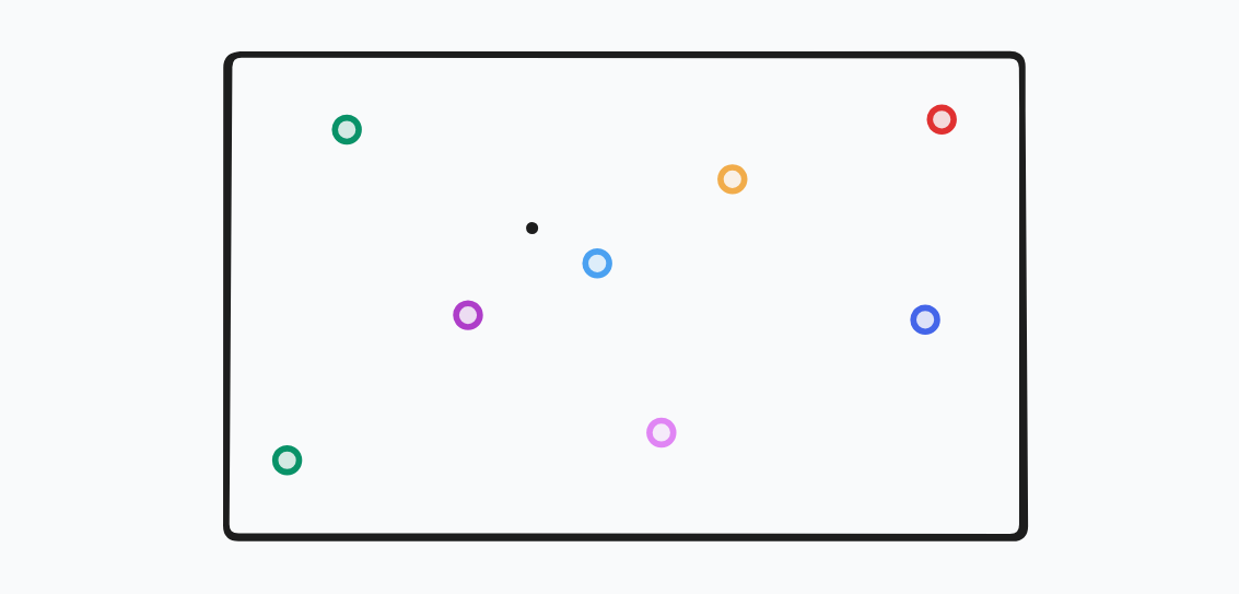
The problem.... is simple to find, really. For the black pixel on the image, we need to find the closest point from the set of points. Looking at the given figure, we know that maybe violet and the blue are the closest ones, but we for sure know that red is not the closest one, in fact, it is the farthest one. So, we need to find a way to not check every point, but only the ones that are close enough to the pixel.
Thankfully, there already exists a data structure specifically for finding nearest neighbours, and it is called a kd-tree.
KD-Tree
It is a kind of a binary tree, which recursively divides a k-dimensional space to allow for effecient querying. So, for example, in a 2D, space, we can first divide the space or the "dataset" vertically (x axis) and then horizontally (y axis) and so on. This continues until we have a tree, where each node represent a region of space.
In our case, we have 2 dimensions, so each node will have two properties, x and y. So in a way, it acts like a alternating binary tree, first we divide by x, then by y, then by x again, and so on.
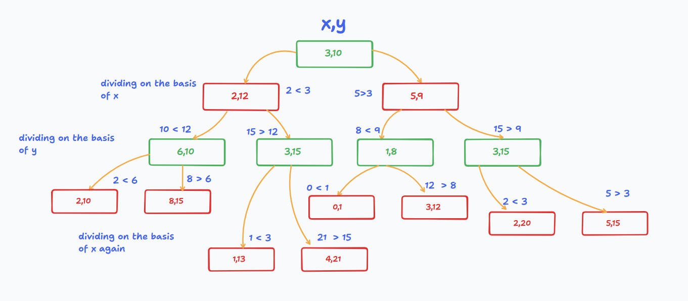
The above diagram, should clear up, how the 2d kd-tree works. But if you are still confused, essentially, in the first layer below the root node, we divided the space by x, i.e the left child has a x value, less than the x value of root node, and the right child has a x value greater than the root node. Then, in the next layer, we divide the space by y, i.e the left child has a y value less than the y value of the parent node, and the right child has a y value greater than the parent node.
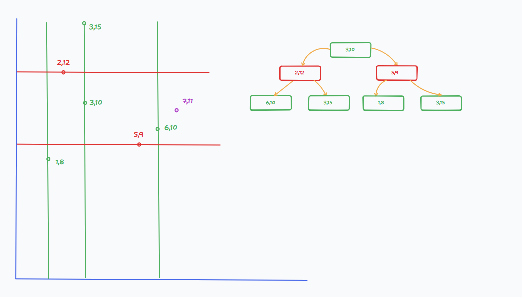
Now to search for the closest point to (7,11). We use the depth of the tree to determine which axis to compare. If we are at an even depth, we compare the x value, and if we are at an odd depth, we compare the y value.
We also need to keep track of the best point we’ve found so far, and the best distance to the point we are searching for. At each step, we calculate the distance from the current node to our target point, and if it’s smaller than the best distance so far, we update both.
We start at the root, which is (3,10) at depth 0. Since the depth is even, we compare x values: 7 (target x) > 3 → we go right to (5,9). Before that, we calculate the distance from (3,10) to (7,11):
So (3,10) becomes our first best point, with distance² = 17.
At (5,9) (depth 1, odd), we now compare y values: 11 > 9 → go right to (3,15). Check distance from (5,9) to (7,11):
So we update our best point to (5,9) with distance² = 8.
Now at (3,15) (depth 2, even), we compare x values again: 7 > 3 → go right, but there's no child. We still compare the distance from (3,15) to (7,11):
This is worse than our current best, so we backtrack to (5,9) and check the left child, which is null, so we backtrack.
And now we perform it recursively, until we find the best point, which in this case is (6,10) with \(distance^2 = 2\).
Here is the code for the nearst neighbour search in a kd-tree:
01pub fn findNearest(self: *const KdTree, target: rl.Vector2, best_dist_sq: *f32, best_index: *usize) void {
02    const dx = target.x - self.point.x;
03    const dy = target.y - self.point.y;
04    const dist_sq = dx * dx + dy * dy;
05
06    if (dist_sq < best_dist_sq.*) {
07        best_dist_sq.* = dist_sq;
08        best_index.* = self.color_index;
09    }
10
11    const axis = self.depth % 2;
12    const target_coord = if (axis == 0) target.x else target.y;
13    const node_coord = if (axis == 0) self.point.x else self.point.y;
14
15    const primary = if (target_coord < node_coord) self.left else self.right;
16    const secondary = if (target_coord < node_coord) self.right else self.left;
17
18    if (primary) |p| {
19        p.findNearest(target, best_dist_sq, best_index);
20    }
21
22    const diff = target_coord - node_coord;
23    if (secondary != null and diff * diff < best_dist_sq.*) {
24        secondary.?.findNearest(target, best_dist_sq, best_index);
25    }
26}
With these enhancements, I was able to generate a 100,000 point map in just 2.9 seconds, which is a 2750x speedup. This is a massive improvement, and I am really happy and content with this result (for now).
We now have some "land", but there is one more thing we need to do before we can start using wfc, and that is to also keep track of the neighbours of each point. This is because, in wave function collapse, we need to know which points are adjacent to each other, so that we can propagate the information correctly. I would also like to store the edges, as I think they will be useful later for river generation.
Neighbours
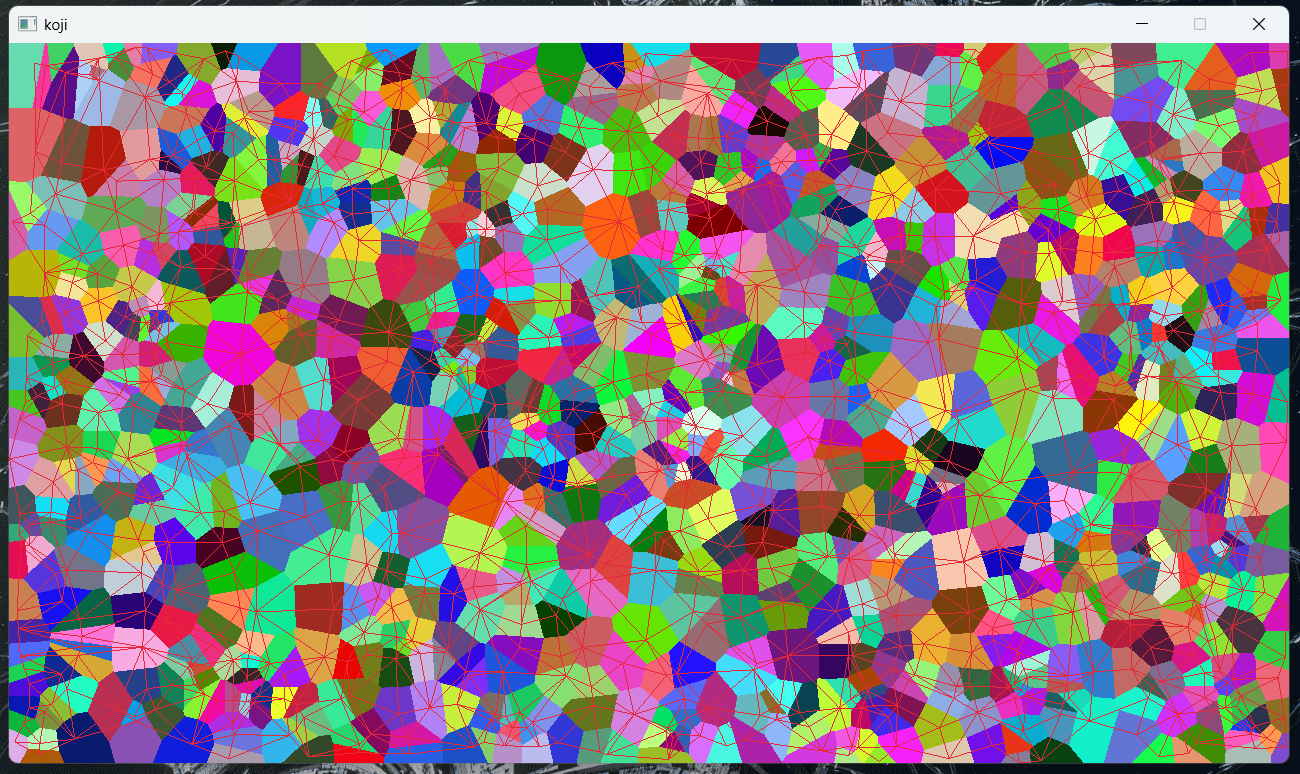
Detecting neighbours involves two steps: direct checking for adjacent points and then using delaunay triangulation. We split the space into a grid. and for a grid, we check its adjacent neighbours. Whenever two adjancent grid cells have different sites, we can detect that they are neighbours. This is a simple and efficient way to find neighbours, and it works well for our use case.
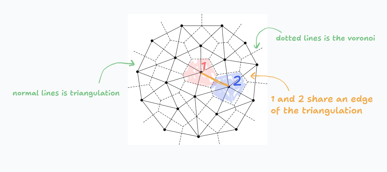
However, rasterized sampling can miss extremely thin adjacency or can be expensive to sample densely. A robust alternative is to compute the Delaunay triangulation. There is a well known fact that Voronoi diagrams are dual to Delaunay triangulations. This means that the edges of the Voronoi diagram correspond to the edges of the Delaunay triangulation, and vice versa or in simpler words, two sites are neighbors in the Voronoi diagram if and only if they are connected by an edge in the Delaunay triangulation
I tried with only using delaunay triangulation, but for some reason, it was leaving a lot of faces out, so I decided to combine both methods, and merge the results. Lot slower, but does give better results.
This works, but the code for it contains a for loop inside a for loop inside a for loop, which is resulting in pretty slow results. I am aiming to have 10,000 tiles in the final version, and this is take 69.8 seconds to generate a map with only 3,000 tiles. So, I need to find a way to make this faster. I need a way that actually just calculates the edges and neighbours while generating the voronoi diagram, instead of doing it after the voronoi diagram is generated. And this is where I discovered Fortune's Sweep Algorithm.
Fortune's Sweep Algorithm
tbd.
Wave Function Collapse
Wave function collapse, at first, seemed like a real complex algorithm, with "superpositions", "entropy" and... somehow quantum mechanics? In reality, it really is not that complex, and the best way to understand it would be to think of a sudoku puzzle.
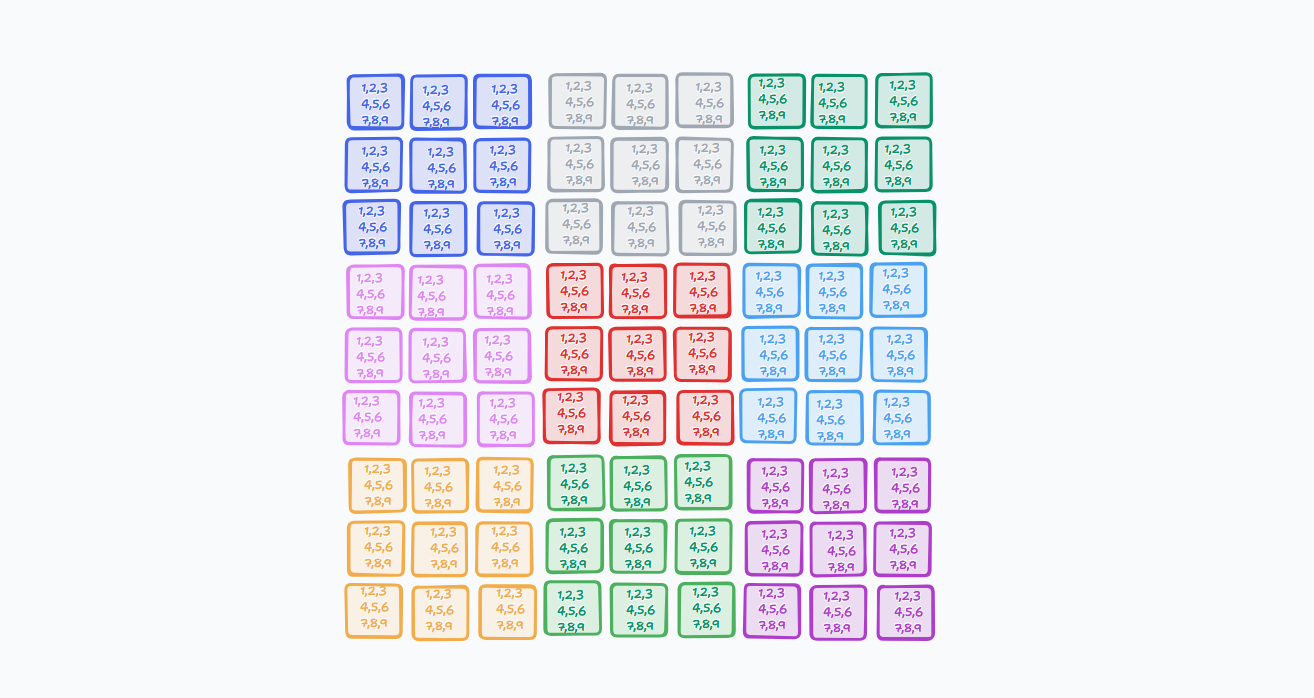
A sudoku, as we all know, is a 9x9 grid, where we need to fill in the numbers from 1 to 9, such that each row, column and 3x3 subgrid contains all the numbers exactly once.
Now, in an empty sudoku, each cell can potentially hold any number from 1 to 9. This is similar to the "superposition" in wave function collapse, where each cell can be in multiple states at once.
But we do know, that sudoku puzzles are not blank, we already have some numbers filled in. These numbers act as constraints, reducing the probabilities for the other cells. For example, if a cell has 5, it cannot have any other number, and now that entire row, column and subgrid cannot have another 5 either. We have "collapsed" the probability of that cell to just one state, which is the number 5. The process of updating the probabilities of the other cells, is called "propagation".
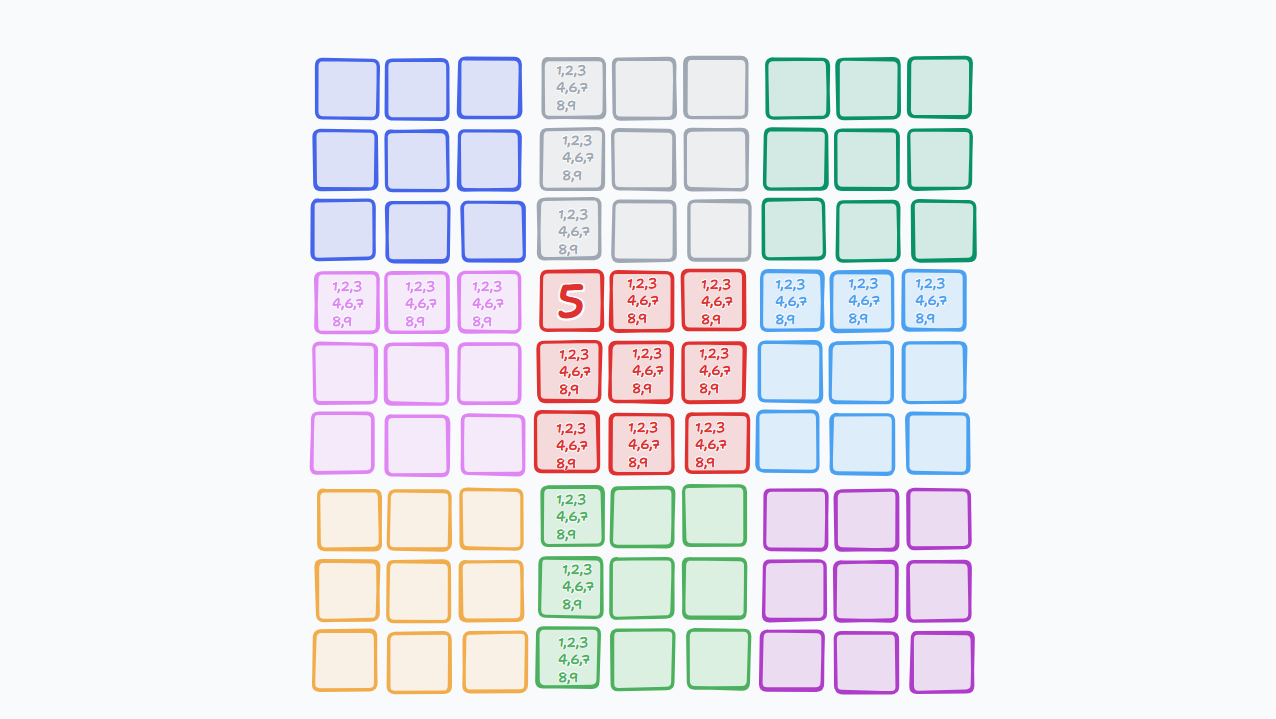
The above image shows how the probabilites change if we add a single number to the sudoku. Now if we add a couple more starting numbers, the probabilities vary even more, with some cells having 3 potential numbers and some still having 9 potential numbers.
Now, to start solving the sudoku, we need to select the cell with the lowest entropy, which here means, the cell with least number of potential numbers, collapse it to a single possibility and propagate the information to affected cells. We now repeat this process until all of the cells are collapsed to a single possibility and the problem is solved!
Now that we understand wave function collapse, somewhat, we can apply it to our map generation.